

One approach to discover structure in data is the use of methods that employ forms of unsupervised competitive learning. The growing neural gas (GNG) proposed by Fritzke [7] is such a method. It belongs to the class of topology representing networks [8]. In contrast to other methods of unsupervised competitive learning, e.g., the self-organizing map (SOM) [9], the GNG does not use a fixed network topology. Instead, the GNG uses a data-driven growth process to approximate the topology of the input space in form of an induced Delaunay triangulation. However, the individual GNG units can only represent local regions of the input space as convex polyhedrons. Hence, complex structures of the input space, e.g., non-convex clusters, can only be approximated piecewise by a larger number of units.
This piecewise representation of input space structures makes it often difficult to recover the relationship between the network units and the corresponding structures in input space. For instance, determining which set of units in the GNG network corresponds to a single, coherent cluster in the input space can be particularly difficult when several other clusters are very close. To support the reconstruction of such relationships, we proposed in [1] an extension to the original GNG algorithm termed local input space histograms (LISH) that adds a local descriptor to each edge of the GNG network. These descriptors then help to characterize the input space structure spanned by the corresponding edges. We show that this descriptor can be utilized in combination with common clustering techniques in order to identify sets of GNG network units that correspond well to non-convex, difficult to separate clusters in the input space.
The growing neural gas uses two mechanisms, edges and accumulated errors, to track how well the network approximates a particular local region of the input space. An edge between two units indicates that the input space between the two units is not empty, and the accumulated error of a unit provides an indication of the relative density of network units with respect to the density of the underlying input space.
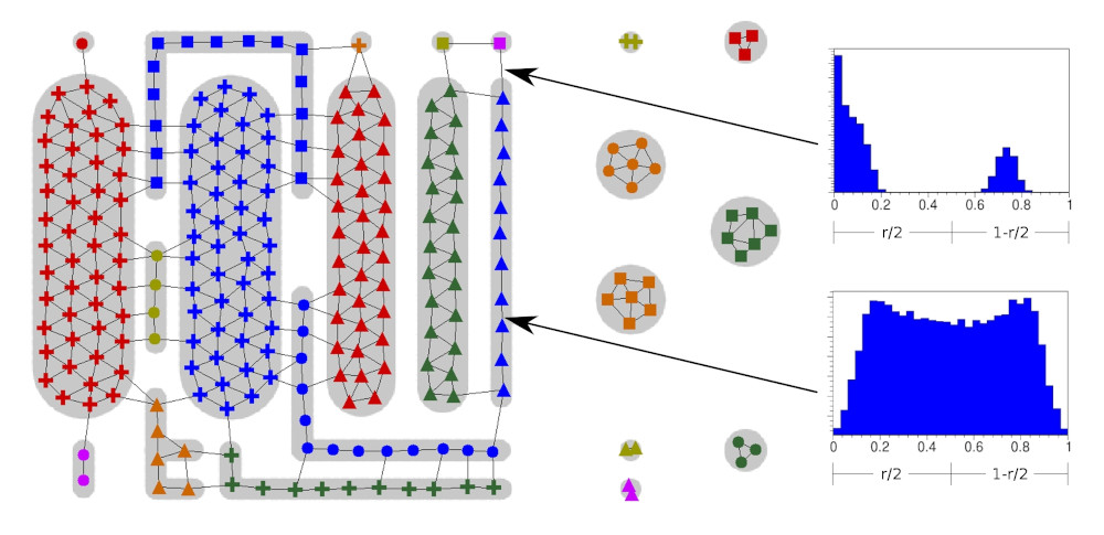
We propose to add a small histogram H to each edge of the GNG network in order to capture more information about the structure of the input space. Every time two nodes connected by an edge are selected as the two units who are closest to an input, the corresponding histogram is updated by using a ratio that captures the relative distance of the input to both units. The resulting histogram captures the local characteristic of the input space that is spanned by the corresponding edge. Figure 1 shows the local histograms of two edges. One of the edges covers a gap in the input space. The other edge spans a region were the inputs are more equally distributed.
Clustering
The additional information that is gathered by the local input space histograms can be used to support the clustering of GNG network units. The basic algorithm uses a plain breadth-first search to identify units that are connected by at least one path. Without any extensions, this breadth-first search identifies isolated sub-networks as individual clusters. This straightforward clustering technique can be extended by deciding for every edge, if the edge should actually be traversed. We propose to use two measures to support this decision: Edges whose information about the input space is uncertain as well as edges that characterize some form of “gap” in the input space should not be traversed. We define the uncertainty of an edge as the average bin error of its histogram H. If the uncertainty of an edge is above a certain threshold, e.g., 10%, the edge will not be traversed. For the second measure we compare the shape of the edge’s histogram with a set of 11 template histograms that represent forms of discontinuous as well as continuous input space. If a histogram matches to one of the templates representing discontinuous input space the corresponding edge will not be traversed.
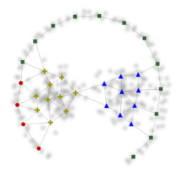
Figure 2 shows the clustering result of an input space with dense regions (light gray) that are partially in close proximity and have non-convex shapes in some cases. In addition, the figure depicts the input space histograms of two edges (black arrows). Although most regions of the input space are connected by edges in their corresponding network representation, the two measures derived from the local input space histograms prevent a merging of the particular clusters.
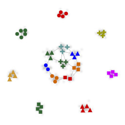
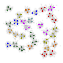
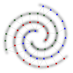
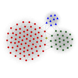
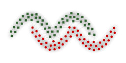
In figure 3 we applied our clustering approach to datasets found in the literature and achieved comparable results. The input spaces in figure 3a and 3b are based on the R15 and D31 datasets in [4], the input spaces in figure 3c and 3d are based on datasets presented in [5], and the input spaces in figure 3e and 3f are based on the datasets shown in [6]. As the datasets of [4] and [5] were given as a set of discrete points, the input spaces were derived by plotting the points as small circles and applying a gaussian filter. In all cases the threshold for the allowed uncertainty of edges was set to 10% and the same set of 11 templates was used.
In two follow-up works we investigated how the LISH approach performs in cases where the input space is high-dimensional and how LISHs can be utilized to form a sparse representation of an input space.
References
1
,
Supporting GNG-based clustering with local input space histograms,
In: Proceedings of the 22nd European Symposium on Artificial Neural Networks, Computational Intelligence and Machine Learning. Louvain-la-Neuve, Belgique, pp. 559–564, 2014,
[pdf|bibtex]
2
,
Analysis of high-dimensional data using local input space histograms,
In: Neurocomputing 169, pp. 272–280, 2015,
[pdf|doi|bibtex]
3
,
A Sparse Representation of High-Dimensional Input Spaces Based on an Augmented Growing Neural Gas,
In: GCAI 2016. 2nd Global Conference on Artificial Intelligence. Vol. 41. EPiC Series in Computing. EasyChair, pp. 303–313, 2016,
[pdf|doi|bibtex]
4
,
A maximum variance cluster algorithm,
In: IEEE Trans. Pattern Anal. Mach. Intell., 24(9):1273–1280, 2002,
[doi]
5
,
Robust path-based spectral clustering,
In: Pattern Recogn., 41(1):191–203, 2008,
[doi]
6
,
The growing neural gas and clustering of large amounts of data,
In: Optical Memory and Neural Networks, 20(4):260–270, 2011,
[doi]
7
,
A growing neural gas network learns topologies,
In: Advances in Neural Information Processing Systems 7, pp. 625–632, MIT Press, 1994,
[details]
8
,
Topology representing networks,
In: Neural Networks, 7:507–522, 1994,
[doi]
9
,
Self-organized formation of topologically correct feature maps,
In: Biological Cybernetics 43(1), 59–69, 1982,
[doi]
10
,
Clustering high-dimensional data: A survey on subspace clustering, pattern-based clustering, and correlation clustering,
In: ACM Trans. Knowl. Discov. Data 3 1:1–1:58, 2009,
[doi]
11
,
On the surprising behavior of distance metrics in high dimensional space,
In: Database Theory — ICDT 2001, Vol. 1973 of Lecture Notes in Computer Science, Springer Berlin Heidelberg, pp. 420–434, 2001,
[doi]