

The recursive growing neural gas (RGNG) algorithm lies at the core of my RGNG grid cell model. In [2] we review the RGNG algorithm and introduce an algorithmic alternative that is structurally less complex, more efficient to compute, and more robust in terms of the input space representation that is learned by the algorithm. The RGNG is an unsupervised learning algorithm that learns a prototype-based representation of a given input space. Although the RGNG is algorithmically similar to well known prototype-based methods of unsupervised learning like the original growing neural gas (GNG) [3,4] or self organizing maps [5], the resulting input space representation is significantly different from common prototype-based approaches. While the latter use single prototype vectors to represent local regions of input space that are pairwise disjoint, the RGNG uses a sparse distributed representation where each point in input space is encoded by a joint ensemble activity.
From a neurobiological perspective an RGNG can be interpreted as describing the behavior of a group of neurons that receives signals from a common input space. Each of the neurons in this group tries to learn a coarse representation of the entire input space while being in competition with one another. This coarse representation consists of a limited number of prototypical input patterns that are learned competitively and stored on separate branches of the neuron’s dendritic tree. The competitive character of the learning process ensures that the prototypical input patterns are distributed across the entire input space and thus form a coarse, pointwise representation of it. In addition to these intra-neuronal processes the inter-neuronal competition on the neuron group level influences the alignment of the individual neuron’s representations. More specifically, the competition between the neurons favors an alignment of the individual representations in such a way that the different representations become pairwise distinct. As a result, the neuron group as a whole forms a dense representation of the input space consisting of the self-similar, coarse representations of its group members. The activity of individual neurons in such a group in response to a given input is ambiguous as it cannot be determined from the outside which of the learned input patterns triggered the neuron’s response. However, the collective activity of all neurons in response to a shared input creates an activity pattern that is highly specific for the given input since it is unlikely that for two different inputs the response of all neurons would be exactly the same.
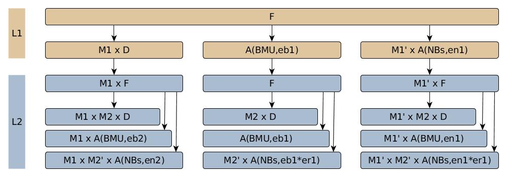
The structure of a RGNG is essentially a multi-layered graph. In case of the RGNG grid cell model two layers L1 and L2 are used. The RGNG graph is dynamic as it grows over time and adjusts its nodes continuously. The dynamic of that change is described by a set of four functions: an input function F, a distance function D, an adaptation function A, and an interpolation function I, where the latter function is only used when the graph grows. The first three functions call each other in a recursive fashion resulting in a non-trivial call graph (Fig. 1) that has to be processed for every input.
The way the RGNG grid cell model forms a distributed, prototype-based representation of the group’s input space is its key aspect. Two main processes are involved in the formation of this representation. First, each neuron has to learn a representation of the entire input space, i.e., it has to distribute the dendritic prototypes it learns across the entire input space. Second, the representations of the individual neurons have to be aligned in such a way that they are pairwise distinct and enable a disambiguation of inputs via the ensemble activity of the neuron group. In the RGNG these two processes depend both on the dynamics encoded in input function F and are controlled by four learning rate parameters, two for each layer. Although the underlying growing neural gas algorithm is relatively robust regarding the choice of learning rates, it can still be difficult to identify a set of learning rates that ensure both the distribution of per-neuron prototypes across the input space and the alignment of the resulting representations such that the overall group-level representation of the input space settles into a stable configuration.
Another important aspect of the RGNG-based model is its computational complexity. For every input the algorithm has to calculate the distance of that input to each prototypical input pattern of every neuron. Since the distance calculation itself is not computationally demanding the RGNG algorithm becomes effectively I/O bound on typical, modern computer systems. When scaling a simulation from individual neuron groups to networks of hundreds or thousands of groups, i.e., exceeding the cache capacity of the system in use the I/O boundedness of the algorithm becomes the main limiting factor of that simulation regarding computation time.
Differential Growing Neural Gas
To address both of the above issues we introduce a novel variation of the growing neural gas algorithm [2], the differential growing neural gas (DGNG), and propose to use it as an approximation of the RGNG algorithm in the context of neuron group modeling. The main idea of the DGNG algorithm is to partition the input space into N regions, where N corresponds to the number of dendritic prototypes that are learned by each neuron. This partition is learned by a top layer growing neural gas with N units representing each input space region by a single prototype vector located at the center of that region. Each region is then partitioned by separate sub-DGNGs into K sub-regions, where K corresponds to the number of neurons in the modeled neuron group. The units of these sub-DGNGs contain prototype vectors that represent a position relative to the center prototype of the corresponding region, i.e., the prototype vectors encode the respective difference between input and center prototype for a given input space sub-region. Compared to the RGNG-based model the correspondence between L1 units and the neurons of the modeled neuron group has been removed in the DGNG. Instead, the representation of each neuron is now distributed among the different sub-DGNGs of the top layer DGNG units. More precisely, the i-th unit of sub-DGNG j contains the j-th prototype of neuron i. Figure 2 illustrates how the different prototype vectors of this new structure are related to one another.
Whereas the distribution and alignment of prototypes in the RGNG algorithm depend on a suitable choice of four different learning rates, the distribution and alignment of prototypes in the DGNG algorithm is directly enforced by its structure, thereby reducing the dependence on suitable learning rates for a particular problem instance. The partitioning of the input space in layer L1 ensures that the coarse input space representations of all neurons always cover the entire input space, while the competition in the L2 sub-DGNGs ensures that the representations learned by each neuron are pairwise distinct. In addition, the partitioning of the input space allows to reduce the number of distance calculations per input significantly.
Modeling of Local Inhibition
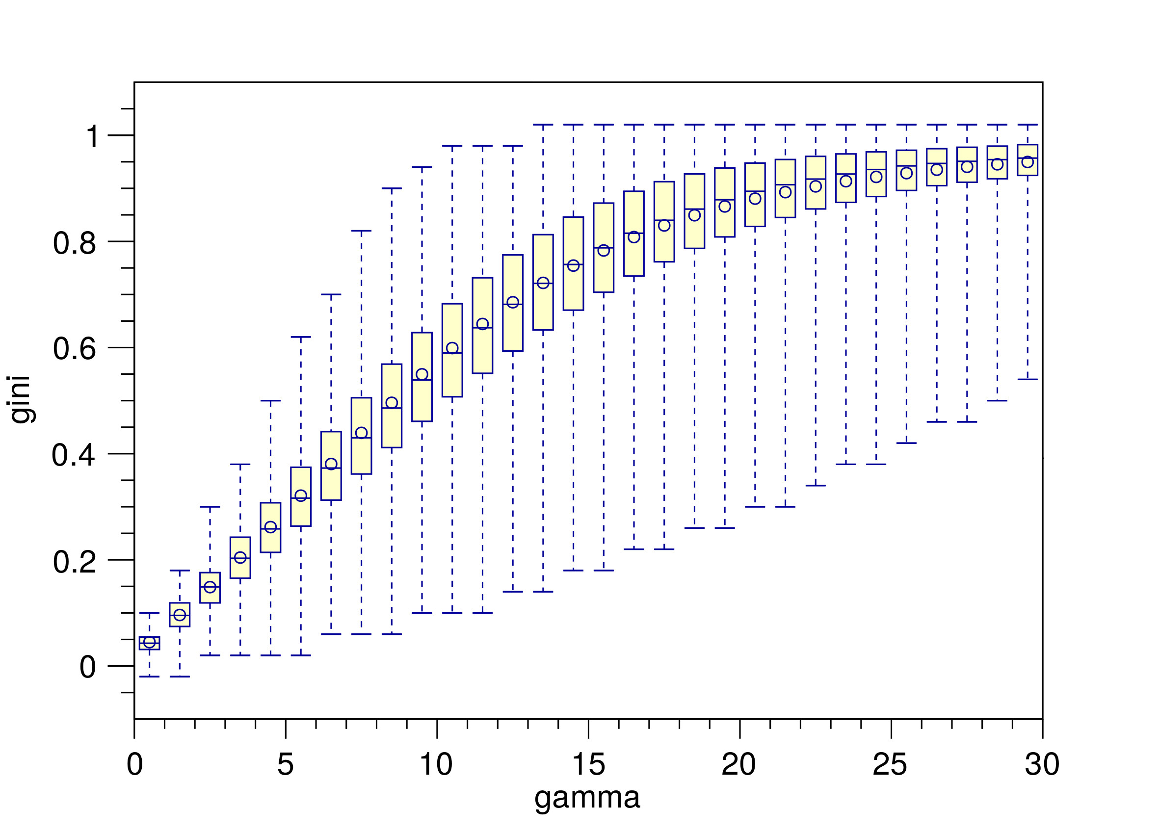
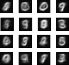
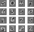
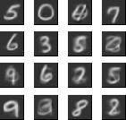
In [2] we highlight an important aspect of both the RGNG and DGNG algorithms. After an input pattern is processed by either a RGNG or DGNG the output of the modeled neuron group is returned as an ensemble activity a that uses a softmax function, which is parameterized by a parameter gamma. This parameter is used to control the degree with which the softmax function emphasizes the largest elements of the ensemble activity a. From a neurobiological perspective the parameter gamma can be interpreted as the strength of the local inhibition that the neurons with the highest activations exert on the other neurons of the group. Figure 3 illustrates the effect of the parameter gamma on the sparsity of the neuron group’s ensemble activity. It shows the distributions of Gini Indices of the ensemble activity vectors in response to input from the MNIST database of handwritten digits [6] in relation to gamma. The Gini Index can be used as a measure for the sparsity of a vector [7]. As an approximation, the value of the Gini Index can be intuitively understood as the fraction of entries in a given vector that have low values (compared to the other entries), i.e., a Gini Index of 0 corresponds to a vector that has similar values in all of its entries whereas a Gini Index of 1 corresponds to a vector that has one or only a few entries with values significantly higher than all other entries of the vector.
The distributions shown in figure 3 illustrates that with increasing values of gamma the mean sparseness of the ensemble activity vectors steadily increases as well. Considering the interpretation of gamma as the degree of local inhibition in the proposed neuron model it becomes evident how important this local inhibition is to the formation of a sparse ensemble code that represents a given input with a sufficient degree of specificity.
The ability to perform such a pattern separation is a key characteristic of the RGNG-based neuron model. To investigate the DGNG-based model in that regard we compared the pairwise cosine similarities of the ensemble activity vectors that were generated in response to the MNIST test dataset. Since the dataset provides labels for the ten different classes of digits it is possible to compare the cosine similarities for intra- and inter-class inputs separately. Given that intra-class samples are likely to be more similar to each other than inter-class samples this distinction of cases allows to study the pattern separation abilities in more detail. In general it is expected that the group of neurons is able to represent individual inputs distinctively in both cases, although the task in the intra-class case is conceivably harder.
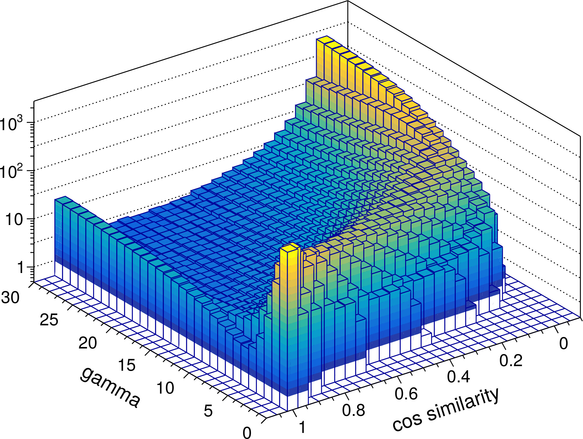
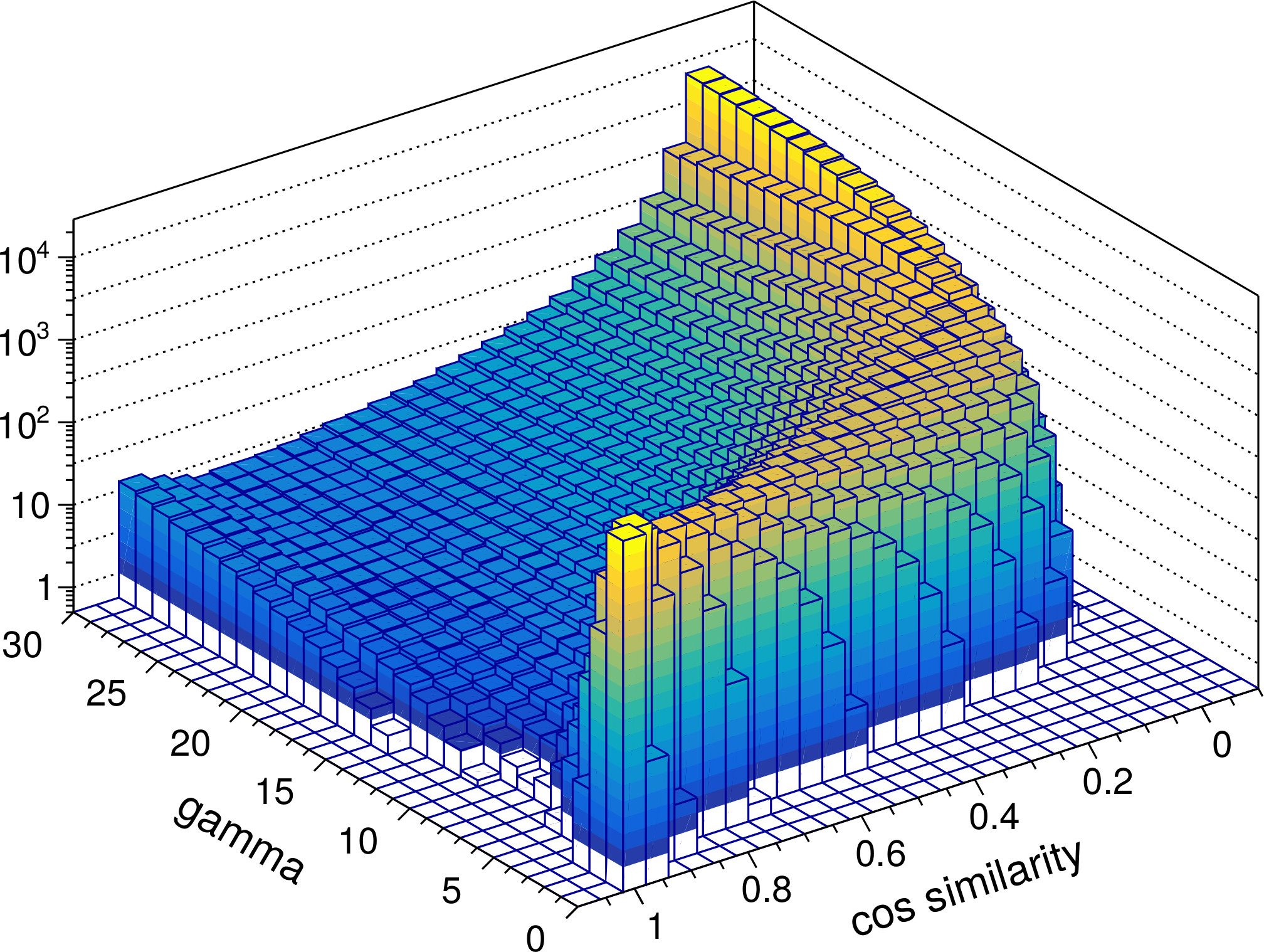
Figure 4 shows the resulting distributions of cosine similarities. In both cases the ensemble activity vectors for values of gamma below 5 are very similar to each other and do not allow to distinguish the neuron group’s responses to different inputs very well emphasizing the importance of local inhibition. However, with increasing values of gamma (≥ 5), i.e., increasing local inhibition, the ensemble activity rapidly becomes very specific. Interestingly, the increase in specificity is not monotonic. The distributions for both intra-class and inter-class samples exhibit a minimum at gamma ≈ 7 and gamma ≈ 5 to 15, respectively. For these values of gamma the response of the neuron group to a given input i is such that very few to none of the other test inputs have a cosine similarity close to 1 with respect to i while the spectrum of occurring, lower cosine similarity values is wide. In contrast, for values of gamma > 15 the distinction between similar or dissimilar inputs becomes much more pronounced. The vast majority of other test inputs (note the logarithmic scale) exhibit cosine similarity values close to 0 in that case, i.e., the corresponding ensemble activity vectors become almost orthogonal to each other.
From a neurobiological perspective the putative ability to shape the characteristic of the neuron group’s input space representation just by the degree of local inhibition alone is a fascinating possibility. It would allow a group of neurons to dynamically switch between fine grained representations that enable the differentiation of very similar inputs and coarse grained, clear-cut representations suitable for fast classification.
References
1
,
A Computational Model of Grid Cells based on a Recursive Growing Neural Gas,
In: PhD thesis. University of Hagen, 2016,
[pdf|bibtex]
2
,
Efficient Approximation of a Recursive Growing Neural Gas,
In: Computational Intelligence: International Joint Conference, IJCCI 2018 Seville, Spain, September 18-20, 2018 Revised Selected Papers, 2021,
[pdf|doi|bibtex]
3
,
A growing neural gas network learns topologies,
In: Advances in Neural Information Processing Systems 7, pp. 625–632, MIT Press, 1994,
[details]
4
,
Unsupervised ontogenetic networks,
In: Handbook of Neural Computation (E. Fiesler and R. Beale, eds.), Institute of Physics Publishing and Oxford University Press, 1996,
[details]
5
,
Self-organized formation of topologically correct feature maps,
In: Biological Cybernetics 43(1), 59–69, 1982,
[doi]
6
,
Gradient-based learning applied to document recognition,
In: Proceedings of the IEEE, 86, 2278-2324, 1998,
[doi]
7
,
Comparing Measures of Sparsity,
In: CoRR, 2008,
[details]