Figure 1: (A) Example of a photo presented to the animal. Yellow traces represent viewing locations recorded by an eye tracker. (B) Example of tracked viewing locations (grey) and recorded cell activity (red) of a single entorhinal neuron (left). Corresponding normalized firing rate map (middle) and rate map autocorrelation (right) of that cell. Maximum firing rate, gridness score (g), and degrees of visual angle (d.v.a.) given above and below figures, respectively. Figure from Killian et al. [2].

Early grid cell research gathered data from a narrow range of experimental paradigms that all involved animals, mostly rats and mice, to move around in simple experimental enclosures [1]. In addition, the subsequent analysis of this data focused on cells with spatially correlated activity while cells that did not meet this criteria were excluded from further investigation. It is possible that this focus reinforced the view that grid cells represent some form of a specialized system for orientation and navigation.

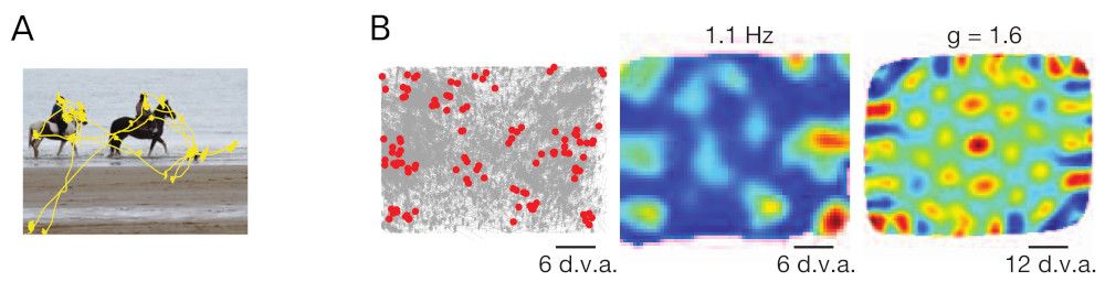
Killian et al. [2] were the first to report grid-like activity from entorhinal cells in an entirely different experimental setting. They investigated the activity of entorhinal cells in primates while the animals sat in front of a computer screen watching photographs. To precisely monitor where the animals were looking the viewing direction was recorded by an eye tracker (Fig. 1a). With this experimental setup Killian et al. found entorhinal cells whose activity correlated with the viewing direction of the animal. Moreover, the cells' firing fields in the animals visual space were arranged in a (coarse) hexagonal pattern (Fig. 1b). These results could not be explained by existing grid cell models as virtually all models were grounded in the prevailing navigation hypothesis using some form of continuous path integration at their core [3]. This continuous path integration could not be mapped on the fast, saccadic eye movements present in these experiments.

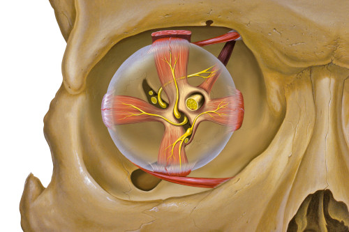
Figure 2: Eye and orbit anatomy with motor nerves by Patrick J. Lynch, medical illustrator; C. Carl Jaffe, MD, cardiologist (CC BY 2.5).

Figure 3: Simulated firing rate maps and distributions of gridness scores for a varying number d of simulated motor neurons per muscle (columns) that control the viewing direction. Each simulated rate map was chosen randomly from the particular set of rate maps and displays all of the respective neuron’s firing fields. The gridness distributions show the gridness scores of all neurons from the particular neuron group.

In contrast, the observations of Killian et al. can be replicated with the RGNG grid cell model if a suitable input space is chosen. Given that the observed neuron activity correlates with locations in visual space the input signal should contain this information. One possible source could be the efference copy from populations of motor neurons that control the eye muscles (Fig. 2). The efference copy of a motor signal is a secondary neuronal pathway that contains the copy of an outgoing signal with which the brain controls a group of muscles. In essence, the efference copy of a motor signal informs other parts of the brain about an intended muscle movement. Individual muscles are usually controlled by a population of motor neurons where the degree of neuronal activity in that population determines the degree of contraction in the particular muscle. Using this simple population code as input to the RGNG grid cell model is sufficient in order to convey enough information about the current viewing direction. Each specific set of population activities corresponds to a specific configuration of eye muscle contractions, which in turn determines the viewing direction. The RGNG grid cell model is able to discover this lower-dimensional manifold of viewing directions in the high-dimensional population code that it received as input.

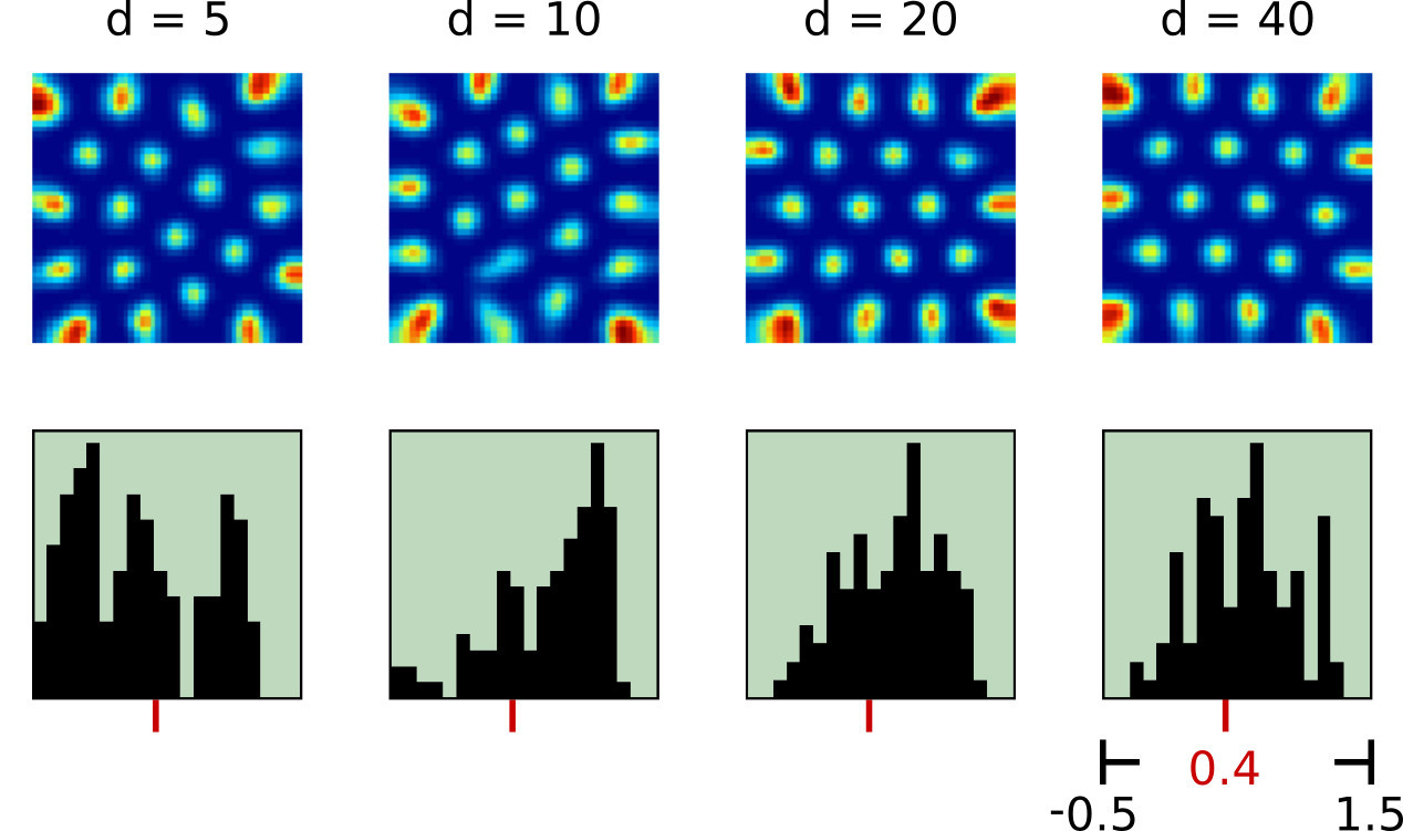
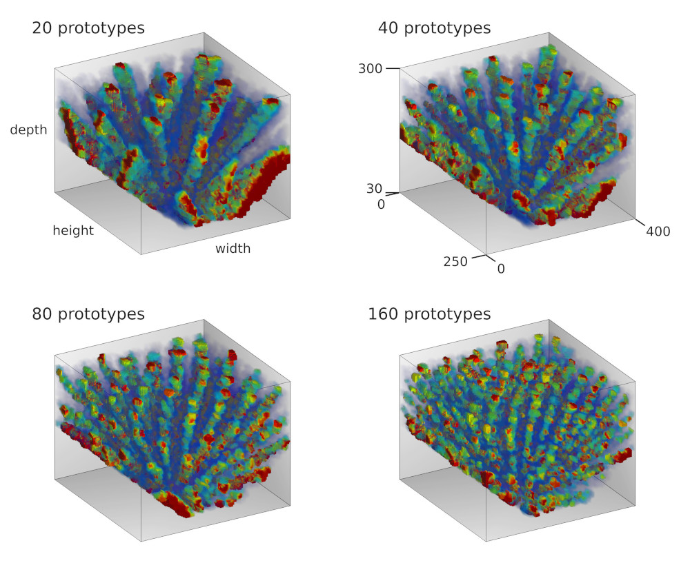
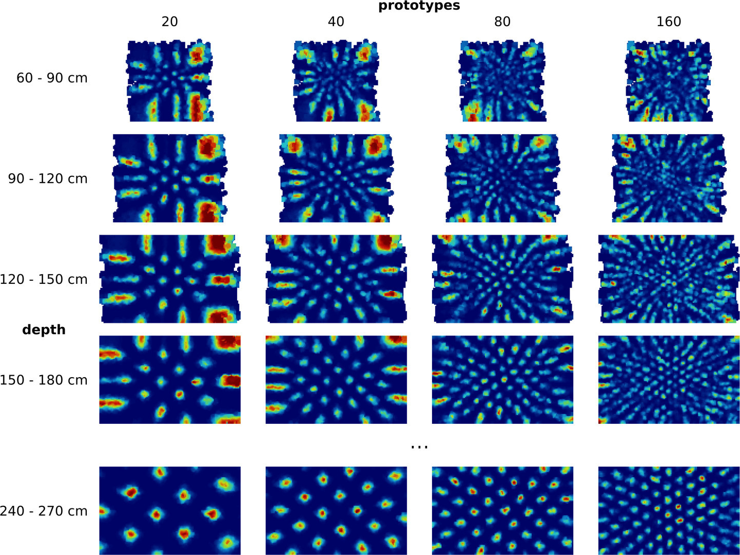
In a first set of experiments we simulated eye movements of one eye and fed the resulting motor signal into the RGNG model [4]. As expected, the model was able to discover the two-dimensional manifold of viewing directions in this input signal resulting in a grid-like distribution of firing fields (Fig. 3). Moreover, the results were relatively consistent across different sizes of motor neuron populations. However, the firing rate maps produced by the model looked significantly cleaner than the firing rate maps reported by Killian et al. [2] (Fig. 1b). This difference might just reflect the inherently difficult experimental conditions when working with primates instead of rodents. In that case, the observed firing rate maps would merely contain more measuring artefacts when compared to similar observations in rats or mice. Yet, the difference could also stem from a different or more elaborate input signal. To investigate this hypothesis we ran a second set of experiments where we simulated the movements of both eyes when fixating on given points in space [5]. As a result, we obtained three-dimensional, volumetric firing rate maps for each simulated neuron (Fig. 4a). The volumetric maps correlate the neuronal activity with points in a three-dimensional view box. We derived two dimensional firing rate maps by slicing through these volumetric maps at given depths (Fig. 4b). To our surprise, the apparent structure of these derived, two-dimensional firing rate maps appears to be more similar to the observed data by Killian et al. [2], especially when a depth range between 60cm and 120cm and a lower number of dendritic prototypes is considered. This depth range agrees with the distance between primate and computer monitor in the experiments of Killian et al. [ personal correspondence ].

(a)

(b)

Figure 2: (a) Volumetric firing rate maps derived from simulation runs with varying numbers of dendritic prototypes {20, 40, 80, 160} per neuron. Each firing rate map was chosen randomly from the respective set of neurons. The rate maps correlate the simulated neuronal activity of a single neuron with the corresponding fixation point within the view box. Eyes are located at the center of the width and height dimensions looking upwards in the direction of the depth dimension. Normalized neuronal activity is color-coded from blue-transparent (low activity) to red-opaque (high activity). (b) Horizontal slices through the volumetric firing rate maps shown in (a). Each slice integrates a depth range of 30 cm. Normalized neuronal activity is color-coded from blue (low activity) to red (high activity). Regions with no data points are drawn in white.

References

1 Jochen Kerdels and Gabriele Peters,
A Survey of Entorhinal Grid Cell Properties,
In: arXiv e-prints, arXiv:1810.07429 (Oct. 2018), arXiv:1810.07429. arXiv: 1810.07429 [q-bio.NC], 2018,
[pdf|bibtex]

2 Nathaniel J. Killian, Michael J. Jutras, and Elizabeth A. Buffalo,
A map of visual space in the primate entorhinal cortex,
In: Nature, 491(7426):761–764, 11, 2012,
[doi]

3 Jochen Kerdels,
A Computational Model of Grid Cells based on a Recursive Growing Neural Gas,
In: PhD thesis. University of Hagen, 2016,
[pdf|bibtex]

4 Jochen Kerdels and Gabriele Peters,
Modelling the Grid-like Encoding of Visual Space in Primates,
In: Proceedings of the 8th International Joint Conference on Computational Intelligence, IJCCI 2016, Volume 3: NCTA, Porto, Portugal, November 9-11, pp. 42–49, 2016,
[pdf|doi|bibtex] best paper award

5 Jochen Kerdels and Gabriele Peters,
A Possible Encoding of 3D Visual Space in Primates,
In: Computational Intelligence: International Joint Conference, IJCCI 2016 Porto, Portugal, November 9–11, 2016 Revised Selected Papers. Cham: Springer International Publishing, pp. 277–295, 2019,
[pdf|doi|bibtex]