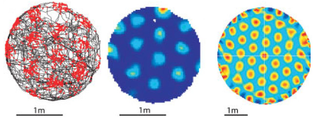
Grid cells are neurons in the entorhinal cortex that exhibit a peculiar form of spatially correlated activity. Mapping the activity of a grid cell to locations in the environment results in a hexagonal grid of firing fields that spans the entire environment (Fig. 1). This prominent characteristic led to the early and prevailing adoption of the idea that grid cells provide some kind of metric for space [1] within a system for orientation and navigation. Accordingly, the vast majority of computational models describe grid cells within this context and rely on (often implicit) assumptions connected to that idea [2,3,4,5,6,7]. However, more recent experimental observations suggest that the activity observed in grid cells might be the result of a more general computational principle that governs the behavior of a much wider range of neurons [8,9,10,11,12,13,14].

To describe the behavior of grid cells at a more abstract level a computational model is needed that is agnostic to the semantic interpretation of its own state and its respective input space such that the model can provide an explanation of the cell’s behavior that does not rely on assumptions based on the putative purpose of that cell, e.g., performing path integration or representing a coordinate system. This way, the observed behavior of grid cells can be treated as just one instance of a more general information processing scheme. To begin, let’s interpret the input signals that a grid cell receives within a small time window as a single sample from a high-dimensional input space. This input space represents all possible inputs to the grid cell and for a certain subset of these inputs, i.e., for inputs from certain regions of that input space the grid cell will fire. We can then split the problem of modeling grid cell behavior into two independent sub-problems:

1. How does a cell choose the regions of input space for which it will fire, given an arbitrary input space?
2. How must a specific input space be structured in order to evoke the actual firing pattern observed in grid cells?

Neuronal models like the well-known Perceptron [15] decribe neurons as simple integrate and fire units. In their case, sub-problem 1 is reduced to a single hyperplane per neuron that cuts the input space in two. For inputs lying on one side of the hyperplane a neuron will fire while for inputs lying on the other side it will remain silent. To model the behavior of grid cells with such a simple neuron model would imply that the grid cell’s input space had to be heavily processed already. The input space would have to have a shape that supports the production of periodic, hexagonally arranged firing fields through a single hyperplane division. Although theoretically possible, it seems unlikely to be the case in practise given the required complexity of the resulting model.

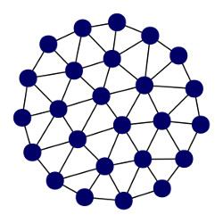
Going back to the grid cell’s firing fields, it is noteworthy how their triangular structure resembles the outcome of computational processes that perform some form of error minimization (Fig. 2). In particular, their structure resembles the structures created by unsupervised, prototype-based learning algorithms. These algorithms form a representation of an input space by distributing a set of prototypes or reference vectors across the input space according to its density, i.e., by placing prototypes in those locations where most inputs come from. We can transfer this basic idea into the realm of biological neurons if we assume that:

• a neuron is able to learn and recognize multiple, different input patterns within its dendritic tree,
• it does so in such a way that it maximizes its activity over all inputs it receives, while
• it is in competition with neighboring neurons.

These assumptions are the three main assumptions on which the grid cell model described below is based on. The first assumption appears to be supported by experimental evidence of Jia et al. [16], Chen et al. [17], and Euler et al. [18]. The second assumption can be motivated by work of Lundgaard et al. [22]. The third assumption is justified by the well-established phenomenon of local inhibition [23].

RGNG Grid Cell Model

A group of neurons exhibiting a behavior that aligns with the aforementioned assumptions can be modeled by a (two layer) recursive growing neural gas (RGNG) [2]. A RGNG is a recursive variant of the growing neural gas introduced by Bernd Fritzke [19,20]. A growing neural gas (GNG) uses a data-driven growth process to approximate the topology of a given input space resulting in an induced Delaunay triangulation of that space. Figure 2 shows an example of a GNG network approximating a uniformly distributed, two-dimensional, circular input space. Each GNG unit marks the center of a convex polyhedron representing a local region of the input space. The relative size of this region is inversely proportional to the probability of an input originating from that region, i.e., the local density of the input space. In addition, the absolute size of each local region is determined by the overall number of GNG units that are available to cover the whole input space. The network structure of the GNG, which relates the respective local regions to one another, represents the input space topology.

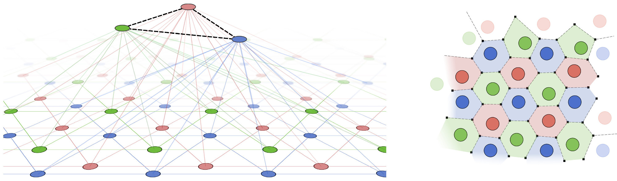
In the RGNG-based grid cell model each neuron performs an operation that is similar to that of a whole GNG, i.e., each neuron learns a prototype-based, dendritic representation of its entire input space. At the same time, each neuron is in competition with the other neurons of its neuron group. This group-level competition is necessary to account for the modular organization of grid cells in which neighboring grid cells share a common orientation, spacing, and field size and exhibit a uniform distribution of relative grid phases. Interestingly, both the learning of a prototype-based input space representation and the group-level competition can be described by the same dynamics. In the two-layer, RGNG-based grid cell model the top layer contains a set of connected units that each represent an individual grid cell. Associated with each top layer unit is a set of connected nodes in the bottom layer representing the set of input patterns that are recognized by the dendritic tree of the grid cell (Fig. 3 left). Applying a form of competitive hebbian learning within each set of bottom layer nodes (bottom layer competition) arranges the nodes in a triangular pattern that covers the entire input space. In addition, competition across the sets of bottom layer nodes (top layer competition) arranges the different triangular patterns in such a way that they share a common orientation and spacing. Furthermore, the top layer competition promotes the uniform spread of the individual triangular patterns across the input space (Fig. 3 right). As a result, the group of neurons described by this RGNG-based model forms a distributed, prototype-based representation of their input space. Each location in that space is represented by a unique pattern of neuronal group activity (ensemble activity) despite the fact that the activity of each neuron itself is ambiguous and self-similar to that of its peers.

Where neural network models based on simple integrate and fire neurons use cascades of hyperplanes to fence in individual regions of input space the RGNG-based model places prototypes directly onto the (typically) lower-dimensional manifold of interest within the input space. As a consequence, the relation between the different prototypes allows to deduce certain topological properties of this input space manifold. In the case of grid cells, for example, the regular hexagonal arrangement of firing fields indicates that the underlying input space manifold is likely to be two-dimensional, uniformly distributed and possibly periodic. These properties hold independent of the actual makeup of the neuronal circuitry that produces the associated input space signals.

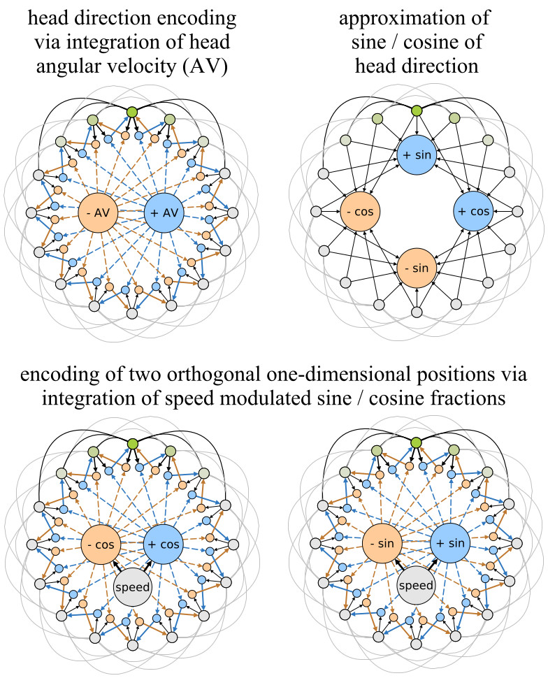
One possible neuronal circuitry that could produce input signals that originate from such a two-dimensional manifold can be derived from ideas by Mc-Naughton et al. [24]. They use one-dimensional attractor networks to explain how the activity of head-direction cells can result from neural integration of angular velocity signals coming from the vestibular system. Figure 4 (top-left) depicts such a model. The outer ring of units represents head-direction cells. They have excitatory connections to neighbouring cells that decline in strength with distance (outer black and grey lines). In addition the set of head-direction cells is subject to global feedback inhibition to constrain the overall neural activity. Typically, such a network forms a single “bump” of activity at one location (green colors). This bump can be moved by a set of hidden units (blue and yellow ochre) that are asymmetrically connected to the outer units. The hidden units receive excitatory inputs from the outer units and from an input unit, e.g., an angular velocity (+/- AV) signal. As a result the angular velocity signal is effectively integrated by the position of the outer bump of activity. In order to transform this head-direction signal into two orthogonal one-dimensional position signals the sine and cosine fractions of the particular head directions have to be approximated. This approximation can be achieved by utilizing a well-known electrotonic property of neurons. The more distant from the soma an axonal input to a dendritic tree is, the weaker is its total effect on the neuron’s activity [24]. Figure 4 (top-right) illustrates, how this property can be used to approximate the sine and cosine fractions of the current head direction. Using the sine and cosine fractions and modulating them with the current running speed of the animal, the same mechanism described for the integration of angular velocity signals can be used to generate two orthogonal, one-dimensional position signals (Fig. 4 bottom). The resulting high-dimensional input to the RGNG-based grid cell model will cause the modeled grid cells to exhibit their characteristic firing patterns as the underlying manifold is a two-dimensional, uniformly distributed, and periodic representation of space. It is important to note that the described input space signal is just one possible neuronal circuit of many.

Results

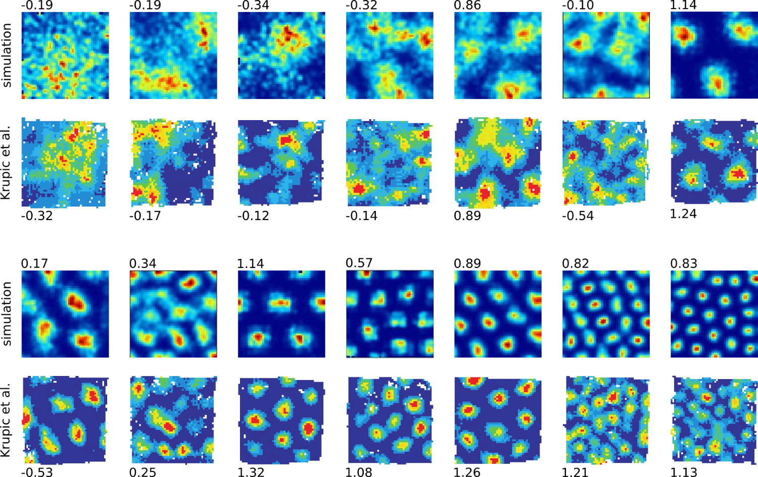
Figure 5 shows the result of some baseline experiments that qualitatively compare the firing rate maps of simulated and observed grid cells (observational data from Krupic et al. [25]). The RGNG-based grid cell model captures a wide range of characteristics that can be found in biological grid cells including “smeared out” firing fields. In the RGNG-based model these smeared out fields result from ongoing micro-adaptations of the dendritic prototype patterns during the integration window in which the firing rate maps were captured. It is plausible that a similar form of micro-adaptation might also occur within the observed, biological grid cells. Corresponding changes in the firing patterns were reported by Krupic et al. [25]).

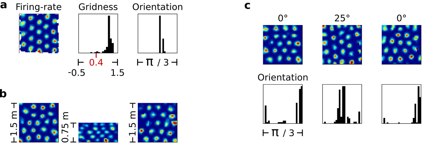
Further computational experiments assessed the RGNG model’s ability to replicate a number of defining grid cell phenomena. For these experiments recorded movement data from the Moser lab was used as input to the RGNG model in order to simulate the movement of an imaginary rat as realistically as possible. Figure 6 shows three example of typical experimental outcomes. Subfigure 6a shows the firing rate map of one grid cell of the simulated grid cell group. Next to the rate map a distribution of gridness scores present in the grid cell group is shown. Gridness scores were introduced by Hafting et al. [21]) to assess whether an observed cell is a grid cell or not. Cells with a gridness score above 0.4 are generally interpreted as grid cells. As the distribution in figure 6a shows most of the simulated neurons achieved gridness scores well beyond this threshold. Next to the distribution of gridness scores a distribution of grid orientations is shown. It indicates a strong alignment of grid orientations in the simulated grid cell group that matches the strong alignment of grid orientations typically seen in observational data.

Figure 6b illustrates the results that were achieved when replicating the phenomena of grid rescaling [26]). Grid rescaling occurs when the size of the experimental environment is suddenly changed. In such a case, the observed grid cell pattern matches the environmental change by compressing accordingly. If the change is reverted, the grid cell pattern returns to its original shape as well. As shown in figure 6b the RGNG grid cell model is able to behave in a similar fashion. The three firing rate maps belong to a single cell before, during, and after a sudden change in the environment’s size.

Lastly, figure 6c shows how the grid orientations in a group of grid cells can be anchored to an external landmark, replicating the corresponding phenomenon observed in biological grid cells. The left column shows the firing rate map of a single simulated grid cell and the distribution of grid orientations in the entire simulated grid cell group. The middle column shows the corresponding data after an imaginary, simulated landmark was rotated by 25°. The right column shows the data after the landmark was rotated back to its original position. In all three cases the resulting distributions of grid orientations resemble the distributions typically seen in observational data, while the grid patterns themselves remain stable.

Both, the phenomena of rescaling and the phenomena of external orientation anchoring show instantaneous changes in the firing fields of observed grid cells. As such, these fast changes cannot be explained by adaptive processes within the neurons themselves and must originate in rapid, though consistent changes of the input signal. The RGNG-based grid cell model can replicate this behavior as it clearly separates learning and representation of any input space and behaving according to a presumed function that is based on specific characteristics of an input space related to that function. No other current grid cell model has this property [2]). As a consequence, the RGNG grid cell model is currently also the only grid cell model that can replicate the grid-like encoding of visual space observed in primates by Killian et al. [12].

Discussion

Beside its ability to describe important characteristics of grid cell behavior the RGNG model has a number of additional computational as well as neurobiological properties that are of interest. Early results indicate that the distributed encoding of the input space is efficient and has a capacity that is exponential in the number of neurons. Consistent with this high capacity the encoding allows for efficient pattern separation whose degree can be controlled by the degree of local inhibition. In addition, the group-level encoding itself is highly fault tolerant as it is based on the coarser neuron-level encodings that are self-similar among neighboring neurons. Thus, if a neuron dies, the neighboring neurons can compensate for that loss with only minimal adaptation of their dendritic prototypes. The self-similarity of the neuron-level encodings is also advantageous from a biological perspective. It leads to a kind of “load balancing” that averages the overall neuronal activity over all neurons in a neuron group making it metabolically efficient, i.e., there are no neurons that spezialize on some rarely occurring patterns that have to be kept alive without contributing much to the overall processing performed by the neuron group. Lastly, the RGNG model uses only local, unsupervised learning. This makes the model quite biologically plausible in that regard compared to, e.g., models that require some form of backpropagation or other forms of global optimization.

References

 1  Edvard I. Moser and May-Britt Moser,
A metric for space,
In: Hippocampus 18(12), 1142–1156, 2008,
[doi]

 2  Jochen Kerdels,
A Computational Model of Grid Cells based on a Recursive Growing Neural Gas,
In: PhD thesis. University of Hagen, 2016,
[pdf|bibtex]

 3  Peter E. Welinder, Yoram Burak, and Ila R. Fiete,
Grid cells: The position code, neural network models of activity, and the problem of learning,
In: Hippocampus 18(12), 1283–1300, 2008,
[doi]

 4  Lisa M. Giocomo, May-Britt Moser, and Edvard I. Moser,
Computational models of grid cells,
In: Neuron 71(4), 589 – 603, 2011,
[doi]

 5  C. Barry and N. Burgess,
Neural mechanisms of self-location,
In: Current Biology 24(8), R330 – R339, 2014,
[doi]

 6  Yoram Burak,
Spatial coding and attractor dynamics of grid cells in the entorhinal cortex,
In: Current Opinion in Neurobiology 25(0), 169 – 175, 2014,
[doi]

 7  Edvard I. Moser, May-Britt Moser, and Yasser Roudi,
Network mechanisms of grid cells,
In: Philosophical Transactions of the Royal Society B: Biological Sciences 369(1635), 2014,
[doi]

 8  Jose Antonio Perez-Escobar, Olga Kornienko, Patrick Latuske, Laura Kohler, and Kevin Allen,
Visual landmarks sharpen grid cell metric and confer context specificity to neurons of the medial entorhinal cortex,
In: eLife, 5:e16937, 2016,
[doi]

 9  Zoltan Nadasdy, T. Peter Nguyen, Ágoston Török, Jason Y. Shen, Deborah E. Briggs, Pradeep N. Modur, and Robert J. Buchanan,
Context-dependent spatially periodic activity in the human entorhinal cortex,
In: Proceedings of the National Academy of Sciences, 2017,
[doi]

 10  Charlotte N. Boccara, Francesca Sargolini, Veslemoy Hult Thoresen, Trygve Solstad, Menno P. Witter, Edvard I. Moser, and May-Britt Moser,
Grid cells in pre- and parasubiculum,
In: Nat Neurosci, 13(8):987–994, 2010,
[doi]

 11  Joshua Jacobs, Christoph T. Weidemann, Jonathan F. Miller, Alec Solway, John F. Burke, Xue-Xin Wei, Nanthia Suthana, Michael R. Sperling, Ashwini D. Sharan, Itzhak Fried, and Michael J. Kahana,
Direct recordings of grid-like neuronal activity in human spatial navigation,
In: Nat Neurosci, 16(9):1188–1190, 2013,
[doi]

 12  Nathaniel J. Killian, Michael J. Jutras, and Elizabeth A. Buffalo,
A map of visual space in the primate entorhinal cortex,
In: Nature, 491(7426):761–764, 11, 2012,
[doi]

 13  Dmitriy Aronov, Rhino Nevers, and David W. Tank,
Mapping of a non-spatial dimension by the hippocampal & entorhinal circuit,
In: Nature, 543(7647):719–722, 2017,
[doi]

 14  Alexandra O. Constantinescu, Jill X. O’Reilly, and Timothy E. J. Behrens,
Organizing conceptual knowledge in humans with a grid-like code,
In: Science (New York, N.Y.), 352(6292):1464–1468, 2016,
[doi]

 15  Frank Rosenblatt,
The Perceptron: A Probabilistic Model for Information Storage and Organization in the Brain,
In: Psychological Review 65 (6): 386-408, 1958,
[doi]

 16  H. Jia, N. L. Rochefort, X. Chen, and A. Konnerth,
Dendritic organization of sensory input to cortical neurons in vivo,
In: Nature, vol. 464, pp. 1307–1312, 2010,
[doi]

 17  T.-W. Chen, T. J. Wardill, Y. Sun, S. R. Pulver, S. L. Renninger, A. Baohan, E. R. Schreiter, R. A. Kerr, M. B. Orger, V. Jayaraman, L. L. Looger, K. Svoboda, and D. S. Kim,
Ultrasensitive fluorescent proteins for imaging neuronal activity,
In: Nature, vol. 499, pp. 295–300, 2013,
[doi]

 18  T. Euler, P. B. Detwiler, and W. Denk,
Directionally selective calcium signals in dendrites of starburst amacrine cells,
In: Nature, vol. 418, pp. 845–852, 2002,
[doi]

 19  Bernd Fritzke,
A growing neural gas network learns topologies,
In: Advances in Neural Information Processing Systems 7, pp. 625–632, MIT Press, 1994,
[details]

 20  Bernd Fritzke,
Unsupervised ontogenetic networks,
In: Handbook of Neural Computation (E. Fiesler and R. Beale, eds.), Institute of Physics Publishing and Oxford University Press, 1996,
[details]

 21  Torkel Hafting, Marianne Fyhn, Sturla Molden, May-Britt Moser, and Edvard I. Moser,
Microstructure of a spatial map in the entorhinal cortex,
In: Nature, volume 436, pages 801-806, number 7052, 2005,
[doi]

 22  Iben Lundgaard, Baoman Li, Lulu Xie, Hongyi Kang, Simon Sanggaard, John D. R. Haswell, Wei Sun, Siri Goldman, Solomiya Blekot, Michael Nielsen, Takahiro Takano, Rashid Deane, and Maiken Nedergaard,
Direct neuronal glucose uptake heralds activity-dependent increases in cerebral metabolism,
In: Nature Communications volume 6, Article number: 6807, 2015,
[doi]

 23  L. Squire, D. Berg, F.E. Bloom, S. du Lac, A. Ghosh, and N.C. Spitzer,
Fundamental Neuroscience,
In: Elsevier Science, 2008,
[details]

 24  B. L. McNaughton, F. P. Battaglia, O. Jensen, E. I. Moser, and M.-B. Moser,
Path integration and the neural basis of the ’cognitive map’,
In: Nat Rev Neurosci, 7(8):663–678, 2006,
[doi]

 25  Julija Krupic, Neil Burgess, and John O'Keefe,
Neural Representations of Location Composed of Spatially Periodic Bands,
In: Science Vol. 337, Issue 6096, pp. 853-857, 2012,
[doi]

 26  Caswell Barry, Robin Hayman, Neil Burgess, and Kathryn J. Jeffery,
Experience-dependent rescaling of entorhinal grids,
In: Nat Neurosci, 10(6):682–684, 2007,
[doi]